6% Guyton SWR; reflux

[obryanjf]

My take on the 6% Guyton SWR. It does not exist without some serious risk in purchasing power. The 6% SWR paper was on a previous thread a week or 2 ago.

My model and its flaws to get the dirty laundry out; not the same data as Guyton’s, I use Gummy’s, I do not have a monte carlo simulator, I use rolling 40 year periods from 1928 to 2000, when rolls out of 2000 it rolls into 1928 again. This yields 75 periods, and this is similar to FIRECALC except the rolling out piece. I have coded 4 equity asset classes rather then 8, due to not having lots of asset class data and not caring to invest the hour or so to code it. Everything else is my interpretation of Guyton’s description and I believe close to what he intended. The 8 asset classes likely improve the DR model a bit, but I believe not materially.

DYODD: I’m an engineer with a MBA, but not a statistian nor a programmer, just a hack. Take the data with a grain of salt and hopefully someone else will evaluate and confirm. I believe it is pretty close.

The issue I have with the original Guyton model is the lost purchasing power (PP). He tries to evaluate this by calculating a final PP (inflation adjusted; IA) and the sum of all withdrawls (IA).
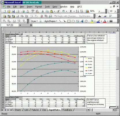
Let me explain the graph. My runs are a 10,20,40,10,10,10,10 (cash, fixed, s&p, small value, large value, small growth) or 10 cash, 20 fixed, 70 equity. No great reason, just my last data check. Now there is a small table on the top and bottom of the graph. The bottom is the total failures for the original Guyton methodology (2006 paper) extended to include his model (DR Model), using the Fixed at retirement model (FIRECALC) and a pure play variable model (x % of previous year net worth).

I think the bottom results are inline with what I would expect. The run is from a withdrawl % (WD%) from 4% to 8% in 0.5% increments. Var model never fails, DR model fails at high WD % because it cannot react fast enough sometimes and fixed is inline with other calculators. Now the top table details when I toggle on failures if the IA withdrawls on a year are less than 50% of the initial withdrawl. Once it fails, that run is a failure, but the run continues, so the end data (averages, etc) would be the same either way. Note if a run fails, the withdrawls sometimes pick up to greater then 50%, but I think 50% is a point I do not what to go during ER. This failure scenerio is one I think Guyton should focus more on.

Note the fixed model runs at a constant IA withdrawl and runs to extinction if foretold by the numbers. The var model and DR model run pretty similar, but ultimately the DR model has more failures at higher WD%.

The graph shows the NPV(sum of all IA withdrawls over a run) and the IA withdrawls averaged. Note the var model works better at lower WD% (4% to 5%) and the DR model at higher WD% (5% to 8%)

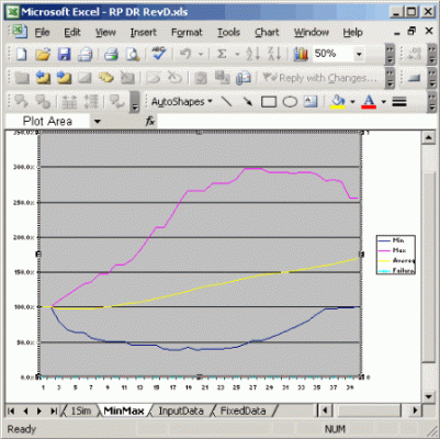
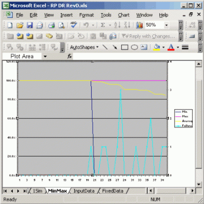
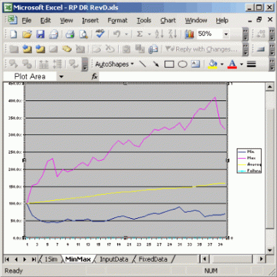
In conclusion: I think the var model provides a better and simpler model for a variable PP withdrawl strategy. Just looking at the end IA WD and the NPV IA WD’s does not do justice to understanding what happens from year 1 to year 40. A failure triggering on <50% (or similar) is key to being able to compare different models. There may be a DR model out there that keeps the PP above some bottom and does not run to extintion, but I do not think this is it.

What will I do? Hope a better DR model emerges by the time I get to critical mass and if not, probably WD about 5% using a var model or a simplier DR model.
Comments?
job

BTW the 64k limit is a pain, that is why the picture is a bit flaky.

 

[2B]

I am pretty familiar with the Guyton article but you lost me.

 

[obryanjf]

What I am saying is using the variable PP model, you may start at say a 6% WD. Say on 1MM port so the WD is 60,000 in todays dollars. Using the rules the WD changes up and down. Sometimes the downs get severe so that the draw per year in inflation adjusted dollards is a pittance of what it was at the start. Below is an example, 6%, 1MM port, 1960 start:

the 4th column is the relavent one which is the inflation adjusted withdrawls. Even though it technically does not fail, the withdrawls at about year 20 or so are < 50% of the initial draw. This would make me pretty nervous about year 15 or so. Also note the inflation adjusted withdrawls eventually recover to almost 100% of the initial withdrawl, but that does not make me feel any better. For 5 years I would have been below 50% and for nearly 25 I would have been barely above 50%.

I think some DR's are good, perhaps even these. My point is his definition of success should be rethought. He defines it just like FIRECALC does which is to run out of money. For a variable PP model this I think is flawed.

job

WD $ percentage Comments WD in IA $
60,000 6.0% 4p R 60,000
60,888 6.4% Inf 6c 4p 60,000
60,888 5.7% Frz 4p 6p R 59,601
61,625 6.5% Inf 6c 12c 4p 59,601
61,625 5.9% Frz 8c 10c 12c 4p 58,627
62,370 5.6% Inf 8c 10c 12c 4p 58,627
63,574 5.2% Inf 4p R 58,627
65,704 5.9% Inf 6c 4p 58,627
67,701 5.1% Inf 10c 12c 14c 4p 58,627
70,897 4.8% Inf 4p R 58,627
75,221 5.9% Inf 6c 8c 4p 58,627
79,344 6.3% Inf 6c 8c 12c 4p 58,627
79,344 6.0% Frz 6c 8c 12c 4p 56,722
82,057 5.8% Inf 4p R 56,722
89,262 7.6% Inf 6c 4p 56,722
80,336 8.8% Cpr 6c 12c 4p 45,499
72,302 6.6% Cpr 8c 10c 12c 4p 38,266
72,302 5.5% Frz 10c 12c 4p 36,507
77,197 6.1% Inf 8c 10c 12c 14c 4p 36,507
77,197 6.0% Frz 8c 10c 12c 14c 4p 33,483
77,197 5.3% Frz 8c 10c 12c 14c 4p 29,547
86,777 5.0% GONEInf 10c 4p 29,547
94,535 5.7% GONEInf 8c 10c 12c 14c 4p 29,547
98,193 5.1% GONEInf 8c 10c 12c 14c 4p 29,547
101,925 4.5% GONEInf 8c 10c 12c 4p 29,547
112,117 4.9% GONEPr 8c 10c 12c 4p 31,246
116,344 4.2% Inf 8c 10c 12c 4p 31,246
127,978 4.2% Pr 8c 4p 33,983
140,776 4.8% Pr 6c 8c 12c 4p 35,803
154,854 4.7% Pr 8c 10c 12c 4p 37,716
170,339 4.5% Pr 4p R 39,648
187,373 5.3% Pr 6c 8c 4p 41,105
193,126 4.6% Inf 8c 14c 4p 41,105
212,438 4.7% Pr 8c 10c 12c 4p 43,886
233,682 4.8% Pr 8c 10c 4p 46,983
239,921 5.3% Inf 6c 8c 10c 12c 14c 4p 46,983
246,327 4.4% Inf 8c 10c 12c 14c 4p 46,983
270,960 4.4% Pr 8c 10c 12c 14c 4p 50,015
298,056 4.0% Pr 8c 12c 4p 54,097
327,862 4.0% Pr 8c 12c 4p 58,570

 

[2B]

I see your point. I wish I understood all of your comments but I think I get most of the idea. I have two comments on it. The first is this is one time period. I would be curious what the average, mean, min and max ranges of adjusted withdrawls over a longer period of starting dates. For a couple of years you got down to 2.95% of the original AI withdrawl. The second point is that if I had started at 4% I would have only had $40,000 in AI dollars and nothing more during this time period. I believe the total case withdrawl is higher even in this less glorious time span.

It's a very interesting analysis.

 

[obryanjf]

The graph shows the total (NPV of WD's IA) and average. The NPV is nothing more than the sum of all the withdrawls over a lifetime simulation and then averaged over the series of years. Each model is a different color(red=var, yellow=DR, green=fixed). The little triangles on the line mean that is the NPV line and the scale is on the right side. The little circles represent the IA WD averages for each run and the scale is on the left. Each model was run for 4%, 4.5%, .. 7.5%, 8% * 75-40 year periods * 40 years.
The second post is a snapshot of a single lifetime sim.
The min and max would be good data to capture. I'll ry it.

job

 

[obryanjf]

Ok, I've done the averages and min_max and I think the results are interesting. I've included the 3 models graphs below. This is 1MM port, at 5% initial draw, same assets and percentages as before. Not sure how they will appear, but they are named fixed, variable and DR. To explain, the min is the lowest of all minimums over the 75 year run for the IA WD as a percentage of the initial WD. The max is similar but the max. The average is the average WD as a percentage of the intial WD for a particular year in the 40 year sim. The failures are the total failures that occured in a particular year for the 75 year run.

I need to think about more but on the DR model i will try to set some maximum adjustment down. Also it appears if the adjustment is sharp and early the portfolio and PP can be saved in the long term. No failures as in the previous run.

On the variable model, it is interesting that the min line is a sharper adjustment down as compared to the DR min line. No failures as expected.

The fixed is as i would expect, a steady average until later in the 40 year sim, some failures start occuring and the average drops. Failures start in the later years in the 40 year sim.

I still like the variable model but will mess around with a sharp, quick adjustment down in the face of conditions that lead to failure. Perhaps I'll also look at when the fixed model fails, what happened to the other models and try to compare.

job

 

[MasterBlaster]

Daddy - O

- First a comment...

Your writing style is very hard to follow. perhaps a few introductory sentences would clear things up.

I'll pass on whether or not the variable model is any good...

However, I'll just notice that using your inflation adjusted numbers that your variable model beat the fixed 4% SWR in all but 11 of the 40 years. Ie withdrawals were > $40k 29 out of 40 years.

My opinion at this time is that the variable withdrawal model represents better what actual retirees do with their stash. When the stash builds up and you've had a good year or two then you'll spend a little more. When the stash is heading downhill fast then you'll tighten up the spending.

Think about it. Are you going to just let your stash build up into millions and millions as you get older and not spend some of it ?

 

[HFWR]

Another suggestion would be to copy the graphs, paste them into Paint or something more elaborate, then save them as jpegs. Would get rid of the Windoze/Exhale toolbars...

 

[obryanjf]

I'll try to write clearer; trying to be concise but thorough on a complicated model. I think I could write volumes on the different permutations I try. Some work and many do not.

The stash building to millions and millions using 4% fixed model is the original problem I had with that model which is why i started to explore other models. I have also a model of a fixed+variable which works well for roughly 2% fixed + 3% to 3.5% variable with very low failure rates.

For the moment, I like the 5% variable model due to simplicity and higher potential WD's along the line.

Simplicity is one thing FIRECALC (fixed model) has going for it for the general populace. To reduce everything down to success rate and a WD rate is key. Most people do not want to think about inflation adjusted averages, standard deviations, triggers for this or that variable, etc.

3 month old wailing, got to go.

job